Page 52 - DJJ20063- Thermodynamics 1

DJJ20063- Thermodynamics 1

INPUT

Interpolation

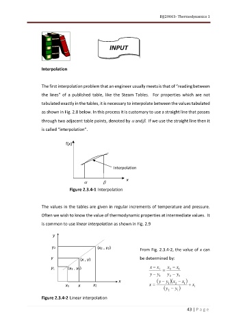
The first interpolation problem that an engineer usually meets is that of “reading between

the lines” of a published table, like the Steam Tables. For properties which are not
tabulated exactly in the tables, it is necessary to interpolate between the values tabulated

as shown in Fig. 2.8 below. In this process it is customary to use a straight line that passes

through two adjacent table points, denoted by  and. If we use the straight line then it

is called “interpolation”.

f(x)

Interpolation

  x

Figure 2.3.4-1 Interpolation

The values in the tables are given in regular increments of temperature and pressure.
Often we wish to know the value of thermodynamic properties at intermediate values. It

is common to use linear interpolation as shown in Fig. 2.9

y

y2 (x2 , y2)
From Fig. 2.3.4-2, the value of x can
y be determined by:
(x , y)

y1 (x1 , y1) x − x 1 = x − x 1
2
y − y y − y
1 2 1
x (y − y 1 )(x − x 1 )
2
x1 x x2 x = ) + x 1
(y − y
2 1
Figure 2.3.4-2 Linear interpolation

43 | P a g e